Overview
An investment’s internal rate of return, or “IRR” is unquestionably the most-quoted north-star metric for expressing performance. While there is no shortage of articles detailing IRR’s theoretical shortfalls, it is extensively used in practice by private equity firms to measure their performance internally and market it externally. When you hear of “top-quartile” PE firms, the determining metric is primarily their latest fund’s IRR.
The runner up in terms of practical usage goes to “MOIC,” which expresses return as a multiple of the invested capital in a deal (hence the name). It is a helpful complement to IRR, but without any information about how long it took the investor to generate. As we know, in this business, time value of money is everything.
All LBO templates will produce an IRR (and typically, an accompanying MOIC), however, thoughtful investors will not accept an IRR figure without an accompanying decomposition of the return into its constituent building blocks. We call this analysis the IRR Decomposition or “IRR Decomp.” for short.
MOICs can also be decomposed in a similar, yet slightly different fashion. MOIC Decompositions are covered in a separate article linked here.
Why Decompose IRR?
If you were presented with two investment opportunities – one showing a 22% IRR, and the other showing a 26% IRR, which would you choose? Would you have follow-up questions?
So would we.
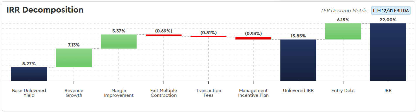
What if we showed you these two charts alongside the question?:
Investment A | 22% IRR
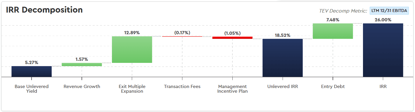
Investment B | 26% IRR
Each component of investment return has varying degrees of associated due diligence and execution risk – and therefore uncertainty – that need to be appropriately reviewed and calibrated when considering the attractiveness of an investment overall.
Extreme examples like the above can be helpful to illustrate a point. Let’s say we had these two investment opportunities presented to us – despite Investment B having a nominally higher IRR, most investors would prefer Investment A because the quality of the IRR – as illustrated by the IRR Decomp – is significantly higher.
In the example above, an investor in Investment B is hoping that the next buyer will pay a materially higher exit multiple in the future than they are considering paying today – put simply, they are betting on exit multiple expansion. Perhaps they have a thesis that they’ve identified a strategic buyer to take them out in five years (a good follow-up question would be “why aren’t they buying it today”…), but typically this IRR Decomp would be met with significant skepticism at Investment Committee.
Investment A, on the other hand, presents an attractive unlevered starting yield (the lowest risk component / most “diligence-able” component of IRR, in this author’s opinion), modest mid-single-digit revenue growth, a clear cost-improvement thesis – which will have execution risk, but can be underwritten with a solid value-creation plan – as well as multiple contraction – i.e., the built-in assumption that the next buyer will pay us a lower valuation in the future than we’re paying today – layering in some conservatism and cushion into the investment (i.e., everything doesn’t have to go perfectly).
Computing the IRR Decomposition
This note discusses Mosaic’s approach to decomposing IRR into industry standard components of investment return. We will begin this discussion by illustrating a standard leveraged buyout transaction whereby the primary entry and exit valuation is framed as a multiple of EBITDA.
This note will also explore how common deal-specific value creation elements impact the IRR Decomp – and how they can be separately isolated – and finally how using nonstandard entry and exit valuation metrics (e.g., ARR, EBITDA less Maintenance Capex, etc.) impacts the mechanics of decomposing IRR.
It is important to note that our methodology is not our invention – but rather a crowd sourced product of thousands of voices from our user base of some of the world’s largest and most successful investors and advisors. By transparently publishing our approach without a paywall, we hope to make industry standard and widely understood what was once opaque, tribal knowledge appreciated by only a small group of practitioners.
Standard IRR Decomp – EBITDA Entry and Exit Multiples
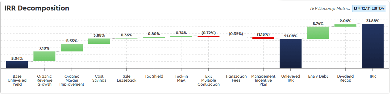
A standard Mosaic LBO will produce an IRR Decomp breaking the deal’s return across the following components as shown in the chart below:
Mechanically, the IRR Decomp is produced by calculating the differences in an investment’s Cumulative IRR before and after each value creation element is layered into the model. This concept is most clearly illustrated on the right-hand side of the chart above by the “Entry Debt” component bridging Unlevered IRR (i.e., our IRR if we used no debt) and our Levered IRR (our IRR including the benefit of debt, commonly just referred to as IRR in the industry).
The IRR Decomp analysis above calculates the 6.15% return attributable to Entry Debt as the difference between the investment’s final cumulative IRR (labeled “IRR” in the chart above at a value of 22.00%) and the cumulative IRR of the investment up until the point we model in leverage (labeled “Unlevered IRR” in the chart above at 15.85%). The remaining components of the IRR Decomp are computed exactly the same way – by sequentially “switching off” the value creation or cost levers shown in the chart above, from right to left, and computing the differences in cumulative IRR before and after each step until all that remains is the “Base Unlevered Yield.”
Mosaic’s automated modeling engine is able to compute iterative calculations like these instantly. In Excel, this analysis is conducted by layering on/off “switches” into each model element you wish to decompose and cycling through them one-by-one as shown below. Mosaic’s Excel download replicates this behavior for those who wish to update their IRR Decomps manually in Excel:
Order Matters
Unlike in the MOIC Decomposition, the order in which you compute an IRR Decomp will determine the value of the IRR impact at each step. This is because IRR is a compounding metric, and therefore the dollar impact of each step will have a different percentage IRR impact depending on the cumulative IRR value immediately preceding it (i.e., that it compounds upon). As such, we must be intentional and consistent about the order in which we compute the IRR Decomp. This note includes our rationale on Mosaic’s order as influenced by discussions with thousands of large-cap private equity investment professionals across our user base.
What is “Base Unlevered Yield”?
The Base Unlevered Yield is the foundation of an investment’s return. It is the IRR you would earn if you bought the business 100% equity-funded (i.e., no debt / “unlevered”) and you generated the starting Unlevered Free Cash Flow of the business – with zero growth – in perpetuity (or exited at a flat exit multiple relative to entry). This figure is a critical component of the IRR Decomp from which each subsequent component builds. Through due diligence of an investment opportunity, investors can build significant confidence in / de-risk this component of the IRR Decomp more readily than subsequent components discussed below. This is because management will have the best visibility into the quality of trailing cash flows (i.e., historical performance) with diminishing confidence in forecast numbers the further out into the future they are. An investor will have an easier time proving that a business can again generate last year’s revenue next year (i.e., they did it once before!) versus underwriting sales in new, unproven initiatives, customer segments, or geographic markets required to grow cash flows.
A Note on LTM vs. NTM Entry Valuation
For models with an LTM (last twelve months) entry valuation metric used, Mosaic frames the IRR Decomp (and thus, Base Unlevered Yield) around the trailing Unlevered Free Cash Flows of the business – holding growth and margin expansion flat from that starting point when computing the Base Unlevered Yield and then attributing IRR to revenue growth and margin expansion. For investors framing their valuation around NTM (next twelve months) entry multiples, we give credit for the NTM growth in the Base Unlevered Yield and downstream IRR Decomp calculations. Our rationale is that if an investor is underwriting an NTM multiple, they believe next year’s earnings are “in the bag” and consider them Base Unlevered Yield. This view was articulated to us by some of the world’s leading software investors who have taken this approach for decades with businesses with a high degree of forward revenue visibility (e.g., subscription revenues).
A Note on Dividending vs. Building Cash
Levered LBOs typically assume free cash flow throughout the investment hold period is used to pay down debt and/or build cash on the balance sheet. In an unlevered investment, however, it would be irrational to hoard free cash flows over a 3-7 year investment period – the rational thing to do would be to pay it out as a dividend to shareholders. This annual “dividending” assumption is also inherent in the unlevered yield metric itself (i.e., your year 1 return would only equal your year 1 unlevered yield if you received that cash flow as a dividend – not if you held it on the balance sheet for multiple years).
As such, we have wired this mechanism into Mosaic’s Base Unlevered Yield – we assume that an investor in an unlevered investment would dividend out any available cash flow each year (i.e., the LBO model assumes a 100% dividend cash sweep for each Unlevered step in the IRR Decomp). This “dividending” mechanism is then reverted to the user’s actual dividend cash sweep assumption for calculating the “leverage” steps in the IRR Decomp (debt or pref), effectively attributing the IRR drag on the timing of cash flows to the use of leverage in the deal. For unlevered investments that do not assume any dividend sweep in the base case (i.e., build cash on the balance sheet until exit), we present this “drag” as a final bridging item labeled “B/S Cash Drag.”
Again, this approach is not our invention, but rather the product of hundreds of conversations with practitioners who have been extremely thoughtful about how they decompose IRR.
Standard Return Levers of the IRR Decomp
Building upon the Base Unlevered Yield, the following are the most common levers of return in a standard private equity investment.
Revenue Growth. This figure expresses how much of the investment’s unlevered return is attributable to the business growing its revenues over the investment hold period. It is computed by layering organic revenue growth into your LBO model on top of the base unlevered yield – but without any of the remaining downstream components of the IRR Decomp. Organic revenue growth is one of the hardest components of an investment to underwrite. We’ve yet to come across a CIM with a negative revenue growth forecast… yet we’ve certainly come across businesses with negative revenue growth…
EBITDA Margin Expansion. This figure expresses how much of the investment’s unlevered return is attributable to the business’ EBITDA margins improving (or degrading) from the outset of the investment to its exit. It is computed by layering on the forecasted margin improvement (or reduction) over the investment hold period. Executing on an organic cost improvement value creation plan is not without risk – however certain private equity firms have built repeatable processes around this motion to reduce execution risk and enhance the “underwritability” of this component.
EBITDA Multiple Expansion (or Contraction). This figure expresses how much of the investment’s unlevered return is attributable to the difference between the valuation multiple paid at entry (i.e., by the initial investor) and at exit (i.e., paid by the next buyer of the asset). For this standard example, we assume that valuation is framed as a multiple of EBITDA at entry and at exit. If a business is purchased for 10x EBITDA and sold for 12x EBITDA, the investment is said to have “two turns of multiple expansion” (which would show up as a positive value in the IRR Decomp), whereas if it is purchased for 10x and sold for 8x, it is said to have two turns of multiple contraction (also sometimes called “compression,” which would show up as a negative value in the IRR Decomp). Recall that in our explanation of base unlevered yield (the initial component), we noted that we assume a flat exit and entry multiple at the beginning of the IRR Decomp analysis. To compute the impact of multiple expansion or contraction, we update the exit multiple to be our modeled exit multiple, recompute the cumulative IRR, and compute the difference between it and the cumulative IRR prior to updating the exit multiple. As discussed in the example above, predicting the outcome of this component of the IRR Decomp is viewed widely as “more luck than skill.” As such, professional investors will rarely bet on exit multiple expansion (i.e., selling at a higher multiple than they bought). It is common to either assume “flat” exit and entry multiples (i.e., equal), or even modest exit multiple compression to err on the side of conservatism.
One-Time Costs. It is standard practice to reflect in base unlevered yield only those revenue and cost components of cash flow that investors deem as “recurring.” In the case of non-recurring, or “one-time” cash costs, it is appropriate to separate them out and layer them in as a separate step of the IRR Decomp, recomputing cumulative IRR before and after their inclusion, and capturing the difference as the contribution (negative) to IRR.
Transaction Fees, Balance Sheet Cash Drag. Mosaic groups together the impact of all non-financing transaction fees into this bucket for a cleaner presentation than showing them separately (considering their immateriality relative to other drivers of return). Also included in this bucket is the IRR impact of cash funded to the balance sheet and minimum cash balance set, if any. Financing fees (i.e., fees incurred to raise debt or pref at entry) are not included here, but rather are included in their respective leverage components of the IRR Decomp.
A Note on Transaction Fees, Cash to Balance Sheet, and Minimum Cash. Often LBOs will assume non-financing transaction fees required to diligence, sign and close a transaction (e.g., legal, accounting, commercial due diligence, etc., typically grouped together as “Transaction Fees”). Further, some investors may assume they will fund some amount of Cash to Balance Sheet at transaction close. These components are typically included in the transaction’s Sources and Uses as well as in the denominator of Unlevered Yield calculations. We refer to a business’ “Fully-Loaded TEV” as the sum of the “Headline” Total Enterprise Value plus these components if applicable. Because these items burden the Unlevered Yield in the denominator, we must calculate them slightly differently in the IRR Decomp. Because they are considered additive to the TEV at entry, a model’s “flat” exit multiple relative to entry is not its headline TEV entry multiple – but rather its Fully-Loaded TEV entry multiple. In Mosaic, we use like-for-like Fully-Loaded TEV multiples in the computation of the multiple expansion / contraction step to appropriately isolate the impact of change in multiple vs. the drag from transaction fees and balance sheet cash. Then, at the step where we compute the impact from transaction fees and balance sheet cash, we turn on the model’s assumed exit multiple (e.g., excluding the impact of fees and cash) to ensure clean attribution to each component. Failing to go through this somewhat pedantic and painful exercise would show, for example, multiple compression in a case where the user’s selected exit multiple was the same as their entry multiple on a headline TEV basis.
Management Incentive Plan. Most private equity deals allocate an options pool or similar incentive to the management team hired to operate the business throughout the investment hold period. Because this money is paid to the management team from the pool of capital that would otherwise be exit proceeds to the investor, we must reflect its impact in the IRR Decomp. This figure therefore expresses how much of the investment’s unlevered IRR is given up to incentivize the management team. Because it is typically tied to the performance of the investment overall, you can expect to see this component be larger for high-performance deals (i.e., high IRR) than for low-performance deals.
Unlevered IRR. The Unlevered IRR is the sum of all the components calculated up to this point. It is also equal to the cumulative IRR with all elements described above included in the model. It is the total return an investor would expect to earn if they acquired the asset with 100% equity (i.e., no debt, or “unlevered”). Unlike the components above, which are presented as “bridging elements” in a waterfall-type chart, the Unlevered IRR is a total element displayed as a helpful interim return before calculating the impact of leverage and the final, levered IRR of the investment.
Entry Debt. This figure expresses how much of the final IRR is generated by using debt at transaction entry to reduce the equity capital required to fund the investment. To compute this value, add to your model the leverage package you are considering and recompute the final, levered IRR of the business. The entry leverage component of the IRR Decomp is simply the difference between the Levered IRR and the Unlevered IRR.
A Note on Prefs. For models in Mosaic that use a combination of Debt and Preferred Equity at entry, Mosaic will show a separate impact for Entry Prefs with the same methodology as described above for Entry Debt.
Levered IRR. The total return generated by the investment opportunity with all elements of the model described above layered in.
IRR Decomp – Non-EBITDA Entry and Exit Multiples
As private equity further institutionalizes as an asset class and value investing techniques are applied to non-traditional LBO candidates (e.g., small, high growth, or even cash-flow negative businesses), creative investors have moved away from cashflow-based valuation metrics towards multiples of Revenue, ARR, or other earnings metrics specific to a certain industry or business model. Doing so modifies the standard IRR Decomp computation and presentation modestly.
Further, investors may choose to value a business at entry on a different valuation metric basis than they do at exit. A common example of this would be for a high-growth, cash flow negative software business – where an investor may value the business on a Revenue multiple basis at entry (when EBITDA is negative), but then on an EBITDA multiple basis at exit (once the business has grown and become EBITDA-positive).
Care must be applied when presenting IRR and MOIC Decompositions for such cases, as decompositions of growth metrics and entry/exit multiples must be conducted on a like-for-like basis (e.g., revenue to revenue, EBITDA to EBITDA, etc.).
Mosaic has a series of built in rules to determine which metric is most logical to decompose a returns bridge based on. First and foremost, if a metric is negative at either entry or exit, is it not a viable candidate to frame the decomposition around, and therefore whichever is consistently positive throughout the investment hold period must be used for the decomposition. In cases where both the entry and the exit metric has a missing data point in either spot, Mosaic reverts to a Revenue-based decomposition as a reliable fallback. For all decompositions, Mosaic clearly identifies in the top-right corner of the analysis what metric the decomposition is framed around.
IRR Decomp – Common Special Situations
The following section covers how Mosaic’s “Special Situations” impact the IRR Decomp analysis. As noted above, order matters in an IRR Decomp, so the team at Mosaic has worked closely with our customers to be thoughtful about the order we’ve selected. The section below describes how special situations are factored into the IRR Decomp in Mosaic and our rationale for determining the order of each component in Mosaic:
“Inorganic” Value Creation Levers
The next group of components following Revenue Growth and Margin Expansion in the IRR Decomposition we consider somewhat “inorganic” – deliberate value creation “plays” authored by a new investor unlikely to be present without external influence. We then order these from most “internal-facing” (e.g., working with assets / resources the company already has) to most “external-facing” initiatives (transactions outside the company / with third parties).
Cost Savings. After factoring in a business’ organic margin improvement, we layer in the impact of any discrete cost savings initiatives included in the value creation plan. Cost savings plays are distinct from organic margin improvement because they typically require one-time costs to achieve a run-rate cost savings target (e.g., advisors, severance expense, etc.). We view this activity as bordering organic and inorganic value creation, and as such compute it first in this group.
Sale Leaseback. The Sale Leaseback value creation lever takes a business’ existing, owned, real estate assets, sells them to a third party, and immediately rents them back from that third party post-close. Leveraging internal assets, but interfacing with external buyers leads us to place this lever’s impact immediately after cost savings.
Tax Shield. Philosophically, we view tax assets (e.g., from step-ups created by the deal) as being inherent to the business but only unlocked as a result of the structuring / set up of the transaction (e.g., basis step ups from asset carve-outs or acquisitions of LLCs). As such, we place them third in the list on the spectrum of most to least “organic.”
Tuck-in M&A. Categorically an inorganic value creation lever, we include next the impact from acquiring many, smaller deals over the course of the investment hold period.
Transformational M&A. The final inorganic value creation lever we include in the IRR Decomp is large, one-off M&A, as the most “inorganic” lever given its outsized potential to transform the very nature of the business that was originally acquired.
A Note on Levered M&A. In the case of an acquisition delayed draw term loan (“DDTL”) being used to fund part of or all M&A, Mosaic’s IRR Decomp will attribute the return benefit of the DDTL to the leverage component of the IRR Decomp by shutting off the DDTL in the unlevered steps of the IRR Decomp.
Rationale for the Order of Remaining Organic Components of Return
There are three or four more organic value contributors that we compute after our set of inorganic value creation plays.
Exit Multiple Expansion (or Contraction). We intentionally leave this value creation lever to this point in the decomposition because it is at this step where we have factored in every other item that could impact the business’ run-rate profitability. For example, M&A increases revenues and EBITDA. Cost savings increase EBITDA, Sale Leasebacks decrease EBITDA. As such, we believe it is logical to compute the impact of the exit multiple expansion or contraction only after all other run-rate earnings-impacting items are incorporated into the analysis – because the change in multiple will impact total EBITDA at the time of exit (organic and inorganic).
One-Time Costs & Exit Fees. Because these are non-recurring in nature, and don’t impact the exit TEV of the business as driven by our assumed exit multiple, we intentionally calculate their impact after the exit multiple expansion, but before the management team’s incentive payout.
Management Incentive Plan. Management’s incentive options or sweet equity are tied to the performance of the investment, including all components covered up until this point. That is why we leave the impact of MIP as the last step of the unlevered IRR bridge. You may argue that the MIP is calculated on a levered return, not an unlevered one – and we would agree – however it is industry standard to calculate the leverage impact as the final step in the IRR Decomp, treating every step prior to that as though the investment was unlevered.
Summary
In summary, the IRR Decomp is an extremely helpful companion analysis to the IRR produced by a standard LBO because of the context it provides about the investment and its sources of opportunity and risk relative to other investment opportunities available today or that have been reviewed in the past. From the above, we can also see that while it is simple in concept, its implementation can be quite complex depending on the investment situation. Inexperienced modelers will frequently miss or skip steps in the IRR Decomp, effectively muddying the Base Unlevered Yield by turning it into a “catch-all” for items not thoughtfully parsed out (e.g., fees, one-time costs, balance sheet cash, etc.). It’s also a perfect example of the case for greater automation and standardization of the modeling workstream. While the output of the IRR Decomp is extremely helpful for deal professionals to consume, its production is a painful, time-consuming exercise in Excel. Time, we’d argue, that’s better spent on commercial due diligence to support or refute the individual components of return you’re underwriting in a given deal, when its automation is readily available in a platform like Mosaic.